CR Decomposition and Inverse Matrices

CR Decomposition

A matrix decomposition is breaking a matrix in several matrices, which usually each give us information about the decomposed matrix. CR decomposition is the first of many matrix decompositions you are going to encounter during the course.

Let’s see why this is true.

• The column space of $A$: C(A) = C(C) : Column space of $C$. This is because we have all linearly independent columns of $A$ in $C$.
• The first point means that we can write the columns of $A$ as a linear combination of the columns of C. This is because the columns of $A$ themselves are also in the column space of A!
• With this point of view, in $R'$ at i-th column, we store how much of which column of $C$ we need to generate the i-th column of $A$.
• We know by Lemma 1.22 that there is only one way of writing a vector as a linear combination of linearly independent vectors. Therefore $R'$ is unique.

$$\underbrace{ \begin{bmatrix} 1 & 3 & 0 & -1 \\ 1 & 3 & 1 & 1 \\ 2 & 6 & 3 & 4 \end{bmatrix} }_{A,\ 3\times 4} = \underbrace{ \begin{bmatrix} 1 & 0 \\ 1 & 1 \\ 2 & 3 \end{bmatrix} }_{C,\ 3\times 2} \underbrace{ \begin{bmatrix} \textcolor{blue}{1} & \textcolor{blue}{3} & 0 & \textcolor{blue}{-1} \\ 0 & 0 & \textcolor{blue}{1} & \textcolor{blue}{2} \end{bmatrix} }_{R',\ 2\times 4}.$$

The $4^{th}$ column of $R'$ tells us that we need $-1$ times the $1^{st}$ column and $2$ times the $2^{nd}$ column of C, in order to generate the $4^{th}$ column of A.

We know that $A$ and $C$ have the same column space. We will see that $A$ and $R'$ have the same row space later. However to convince yourself that $\textbf{R}(A) = \textbf{R}(R')$ now, you can view the matrix multiplication $CR'$ as the linear combination of the rows of $R'$. We have

$$\text{(1st row of A) = 1 }\cdot (\text{1st row of }R') + 0\cdot(\text{2nd row of }R')$$

where the coefficients $1$ and $0$ are the first row of $C$. You use the rows of $R'$ to generate the rows of the matrix $A$ so intuitively we have $\textbf{R}(A) = \textbf{R}(R')$.

Keep in mind: You can also use the $CR$ decomposition to compress the matrices. $A$ has $m\cdot n$ entries whereas you only have to store $(m+n)\cdot r$ entries in the CR-decomposition.

How to calculate CR’ decomposition?

Even though we do did not see an automatized, algorithm based method to calculate the $CR'$ decomposition at this point in the course, you can still eyeball the $CR'$ decomposition in some cases. The $i^{th}$ column of $R'$ tells you how you need to combine the columns of $C$ so that their linear combination gives the $i^{th}$ column of $A$.

A = 130−113112634

C R′ = 1 0 1 1 2 3 1 3 0 −1 0 0 1 2

a ₁ = 112 = 1 · 112 new column of C

a ₂ = 336 = 3 · 112

a ₃ = 013 = 0 · 112 + 1 · 013 new column of C

a ₄ = −114 = (−1) · 112 + 2 · 013

Inverse Matrices

Until now we have seen how to add matrices, how to multiply them, but not how to take back the multiplication by a matrix. If you see a matrix as a linear transformation, this taking back operation would correspond to undoing the effect of the linear transformation. Did your matrix stretch the space and doubled every distance in $x_1$ direction? Then the inverse would shrink the space in the same direction so that everything gets back to “normal”, or in other words everything gets back to the way as they were before you applied the first transformation.

Functions and Bijectivity

Think of $f: X \to Y$. For us to be able to undo the operation, we have to have every possible output coming from exactly one possible input. As you know from other lectures, we call such functions bijective since they are both injective and surjective.

We can make some initial statements about the reversible transformations¹:

• A transformation (function) $T: X \to Y$ is reversible if for every $y\in Y$, there exists exactly one $x\in X$ such that $T(x) = y$. ($\sim$ Def. 2.46)
• The inverse is denoted with $T^{-1}:Y\to X$ and called the inverse or the backward transformation. ($\sim$ Def. 2.46)
• If $T$ is reversible, so is its inverse $T^{-1}$. The inverse of the inverse is the forward transformation itself ie. $(T^{-1})^{-1} = T$, with $T(T^{-1}(y)) = y, \text{ and } T^{-1}(T(x)) = x$. ($\sim$ Fact 2.47)
• The inverse of a reversible linear transformation is also a linear transformation. ($\sim$ Lemma 2.48)
• The inverse of a reversible matrix transformation is also a matrix transformation ($\sim$ Corollary 2.49)

Now we can convince us that a matrix has to be square in order to be undoable. This means in particular that the matrix transformation $T_A: \R^{n}\to \R^{m}$ cannot be bijective if $m\ne n$. Let’s see this for both cases $m < n$ (short and wide matrix) and $n < m$ (skinny and tall matrix).

To see this we can look at an example. You can find the formal proofs (Lemma 2.50 and Lemma 2.51) in the lecture notes.

Case ($m<n$): If we have $m<n$ we have a short and wide matrix with the matrix transformation $T_A: \R^{n} \to \R^{m}$. We are trying to squeeze everything from some higher dimension to some lower dimension. Naturally some things must overlap. So if we try to revert this squeezing we can’t know what goes where. Here is an example with $n=3$ and $m=2$. We are doing projection and transforming $\R^3 \to \R^2$

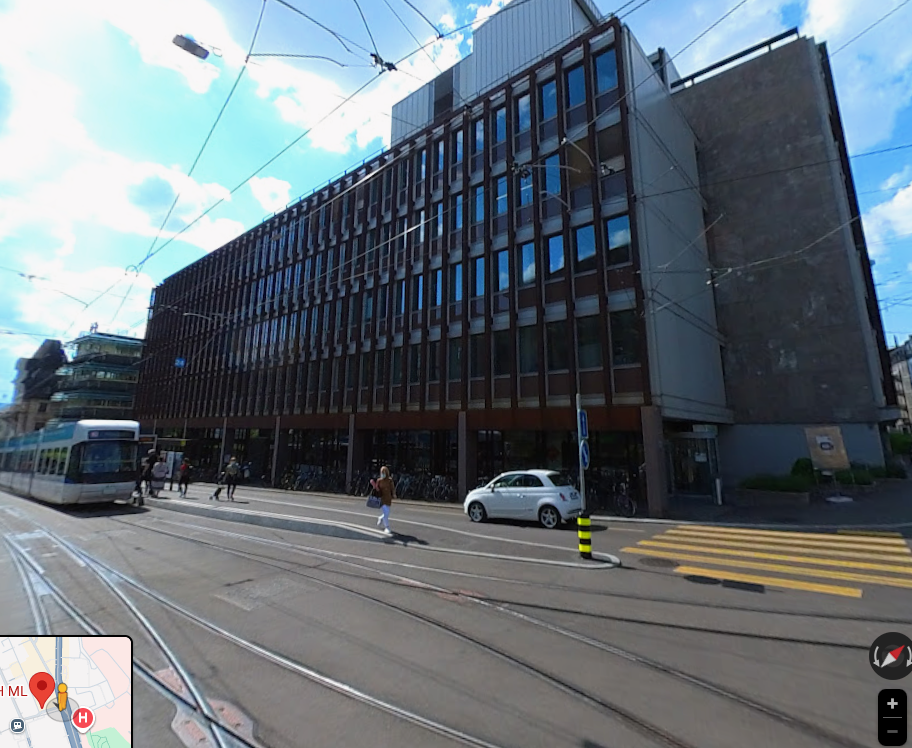
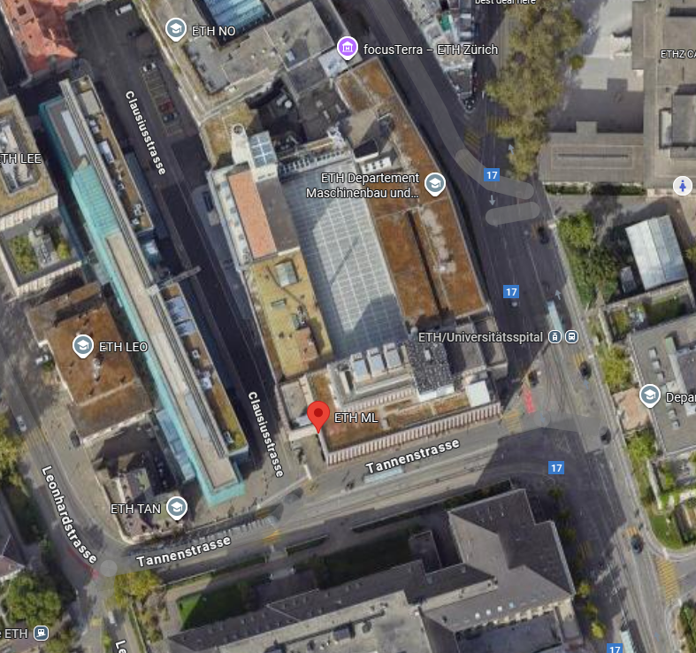
Figure 1: Mapping from a 3D space (left) to its projection in $\mathbb{R}^2$ plane (right).

Now if you are asked to take this operation back just by looking at the 2D image, you wouldn’t be able to do so. For example you can not know how many stories the building has or what color the side facades have. This operation is not injective and hence not bijective (not undoable).

Case ($n < m$): If we have $n < m$ we have a skinny and tall matrix with the matrix transformation $T_A: \R^n \to \R^m$. We are trying to fill out a larger space of $m$ dimensions using inputs from a smaller dimension $n$ but we simply do not have enough input to fill the whole space. This will lead to some parts in the larger output space to have no input mapped to them. Therefore our operation will not be surjective and hence not bijective (not undoable). Here is an example with $n = 2$ and $m = 3$.

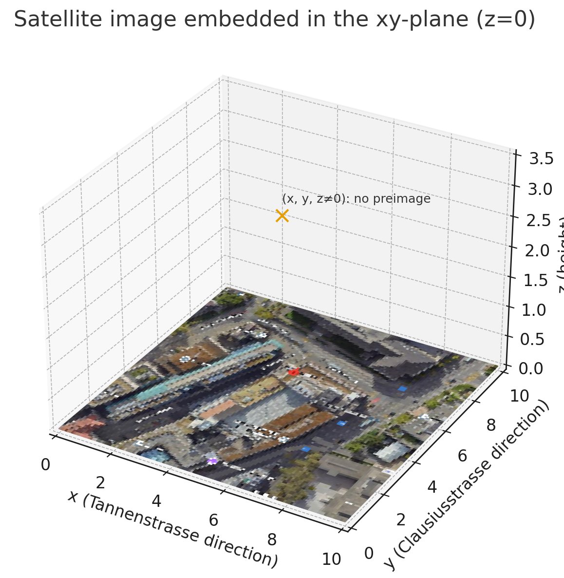
Figure 2: Mapping from a 2D plane (left) to its embedding in $\mathbb{R}^3$ (right).

Now if you were asked to take this operation back for every point in $\R^3$ you wouldn’t be able to do so. This transformation is essentially

$$\begin{pmatrix} x\\y \end{pmatrix} \mapsto \begin{pmatrix} x\\y \\ 0 \end{pmatrix} \text{ with the matrix } \begin{bmatrix} 1 & 0 \\ 0 & 1 \\ 0 & 0 \end{bmatrix}$$

and it is irreversible if you have $z \ne 0$ in the 3D space. As you can see only the xy-plane can be mapped back but the marked point outside of the plane can not be mapped back to the input domain. This operation is not surjective and hence it is not undoable (not bijective).

Keep in mind that these examples are here for intuition. And as the lecture notes say, this intuition does not hold for all the functions. See the formal reasoning in the lecture notes.

Inverse of a Bijective Linear Transformation

Now we know that only linear transformations that can possibly be invertible are the linear transformations $T: \R^m \to \R^m$.

Now we formally state the equivalence we have seen in the previous subsection:

Most importantly we know that the left inverse of an $m\times m$ matrix $A$ is also its right inverse.

The Inverse of a Matrix

Let’s formally define an invertible matrix:

We have further alternative definitions of the invertible matrix:

How to calculate the inverse?

Case $1 \times 1$.

$$M = \begin{bmatrix} a \end{bmatrix} \quad \Rightarrow \quad M^{-1} = \begin{bmatrix} \tfrac{1}{a} \end{bmatrix} \quad (\text{if } a \neq 0).$$

Hence, the inverse exists unless $a = 0$.

Case $2 \times 2$.

$$M = \begin{bmatrix} a & b \\ c & d \end{bmatrix}, \quad \Rightarrow \quad M^{-1} = \frac{1}{ad - bc} \begin{bmatrix} d & -b \\ -c & a \end{bmatrix} \quad (\text{if } ad - bc \neq 0).$$

The inverse for $2\times 2$ matrices exist, if and only if $ad-bc\neq 0$. This is equivalent to say that the inverse of the $2\times 2$ matrix exists, if and only if the columns of it are linearly independent. (Think about this!).

This formula might feel like it came out of nowhere, but these two examples above are only special cases of a general rule to calculate the inverse of a matrix. The formula utilizes some linear algebra tools we have not acquired yet, like determinants and cofactors, but don’t worry, we are going to get there.

Last but not least we list a few important properties of the inverse:

You can find proofs of this facts in the lecture notes but I recommend to think about the proofs before you read them.

Note: An important note to be aware of is that you can not slap $^{-1}$ on top of any matrix when you are doing calculations. You have to know that the matrix $A$ is invertible, before you write $A^{-1}$, because writing $A^{-1}$ is already assuming the inverse exists.

As an example, you should be careful when writing

$$(AB)^{-1} = B^{-1}A^{-1}$$

by Lemma 2.58 The lemma clearly states that this applies when $A$ and $B$ are both invertible. It might be the case that $AB$ is invertible but $A$ or $B$ or both matrices are not invertible by themselves because they are not square matrices. So you should know or show that $B$ and $A$ are invertible, before you can apply this lemma.

Example:

$$A = \begin{bmatrix} 1 & 1 & 3\\ 2 & 0 & 3 \end{bmatrix} \quad B = \begin{bmatrix} 1 & 3\\ 2 & 0 \\ 1 & 1 \end{bmatrix} \quad AB = \begin{bmatrix} 6&6 \\ 5&9 \end{bmatrix}$$

Here $A$ and $B$ are not invertible since they are not square matrices, but $AB$ is invertible.

Hints

1. Solved In Class
2. Solved In Class
3. a) Use associativity b) be careful here $A$ is not necessarily invertible c) no hints
4. No hints.
5. a) use induction over k b) No hints. c) This is a one liner think clever d) you have already seen a type of matrix in the course, which can be a self inverse, find it. (you are of course free to come up with another one) e) If you can modify the one from the previous subtask, go for it.
6. (Challenging) a) use formula b) You have to prove two directions. Drawing a sketch or writing down such a matrix might help. For the proof of one direction, the proof for Theorem 3.7. $\lnot (i) \Rightarrow \lnot (ii)$ might inspire you. c) Assume for a contradiction that the inverse of a lower triangular matrix is not lower triangular. What is the issue here? Argue formally for the general case. d) No hints. You can still do this one without actually solving the first three subtasks.

Footnotes

1. The formal versions of these can be found in the corresponding definitions in the lecture notes ↩