Matrices and Matrix Transformations

Matrices and Linear Combinations

Matrices are a table of real numbers. They can also be seen as a sequence of vectors. But they are more than that. They are functions, they can represent linear systems of equations and they are central to most of the operations in linear algebra. Matrices are images, neural networks, backbone of AI and multidimensional computation.

Definitions

Informally, matrices are rectangular array of (for now, real) numbers. Here is an $m \times n$ matrix:

$$A = \begin{bmatrix} a_{11} & a_{12} & a_{13} & \dots & a_{1n} \\ a_{21} & a_{22} & a_{23} & \dots & a_{2n} \\ \vdots & \vdots & \vdots & \ddots & \vdots \\ a_{m1} & a_{m2} & a_{m3} & \dots & a_{mn} \end{bmatrix}, A \in \mathbb{R}^{m \times n}$$

There are other notations which make writing and understanding the matrices relatively easier.

$$\underbrace{A = \begin{bmatrix} \vert & \vert & & \vert \\ \textbf{v}_1 & \textbf{v}_2 & \dots & \textbf{v}_n \\ \vert & \vert & & \vert \end{bmatrix}}_{\text{Column Notation}} \qquad \underbrace{\begin{bmatrix} \text{---} & \textbf{u}_1 & \text{---} \\ \text{---} & \textbf{u}_2 & \text{---} \\ & \vdots & \\ \text{---} & \textbf{u}_m & \text{---} \end{bmatrix}}_{\text{Row Notation}}$$

Matrix Addition and Scalar Multiplication

Matrix addition and scalar multiplication are defined element-wise. This is why, in order to add two matrices $A$ and $B$ their dimensions must match!

Matrix Addition:

$$\begin{aligned} A + B &= \begin{bmatrix} a_{11} & a_{12} & \dots & a_{1n} \\ a_{21} & a_{22} & \dots & a_{2n} \\ \vdots & \vdots & \ddots & \vdots \\ a_{m1} & a_{m2} & \dots & a_{mn} \end{bmatrix} + \begin{bmatrix} b_{11} & b_{12} & \dots & b_{1n} \\ b_{21} & b_{22} & \dots & b_{2n} \\ \vdots & \vdots & \ddots & \vdots \\ b_{m1} & b_{m2} & \dots & b_{mn} \end{bmatrix} \\[1em] &= \begin{bmatrix} a_{11}+b_{11} & a_{12}+b_{12} & \dots & a_{1n}+b_{1n} \\ a_{21}+b_{21} & a_{22}+b_{22} & \dots & a_{2n}+b_{2n} \\ \vdots & \vdots & \ddots & \vdots \\ a_{m1}+b_{m1} & a_{m2}+b_{m2} & \dots & a_{mn}+b_{mn} \end{bmatrix} \end{aligned}$$

Scalar Multiplication:

$$\lambda \cdot A = \begin{bmatrix} \lambda \cdot a_{11} & \lambda \cdot a_{12} & \dots & \lambda \cdot a_{1n} \\ \lambda \cdot a_{21} & \lambda \cdot a_{22} & \dots & \lambda \cdot a_{2n} \\ \vdots & \vdots & \ddots & \vdots \\ \lambda \cdot a_{m1} & \lambda \cdot a_{m2} & \dots & \lambda \cdot a_{mn} \end{bmatrix}$$

Matrix Shapes

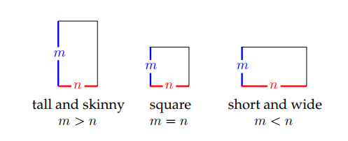
The names that we came up with to describe the matrices might sound funny but they tell us a lot about the matrix. For now just be aware of the intuitive names:

from the lecture notes HS25

Square Matrices

Square matrices are special for reasons that will become clear later. We have specific and intuitive names to describe specific square matrices as you can see below. Be aware that a non square matrix can not belong to one of these categories.

$$\begin{array}{ccccc} \begin{bmatrix} 1 & 0 & 0 \\ 0 & 1 & 0 \\ 0 & 0 & 1 \end{bmatrix} & \begin{bmatrix} 2 & 0 & 0 \\ 0 & 4 & 0 \\ 0 & 0 & 5 \end{bmatrix} & \begin{bmatrix} 2 & 1 & 0 \\ 0 & 4 & 7 \\ 0 & 0 & 5 \end{bmatrix} & \begin{bmatrix} 2 & 0 & 0 \\ 1 & 4 & 0 \\ 0 & 7 & 5 \end{bmatrix} & \begin{bmatrix} 2 & 1 & 0 \\ 1 & 4 & 7 \\ 0 & 7 & 5 \end{bmatrix} \\[1em] \text{identity} & \text{diagonal} & \text{upper triangular} & \text{lower triangular} & \text{symmetric} \\ \text{matrix} & \text{matrix} & \text{matrix} & \text{matrix} & \text{matrix} \end{array}$$

Examples from lecture notes p.46

Formal definitions can be found in the lecture notes. A square matrix can be attributed with more than one of the features listed above. For example a diagonal matrix is an upper triangular and also a lower triangular matrix, it is symmetric as well. E.g. a zero matrix has all four features together.

Matrix Vector Multiplication

Matrix vector multiplication can be seen as the linear combination of the columns of the matrix, where the coefficients are the elements of the vector.

$$2 \begin{bmatrix} 1 \\ 3 \\ 4 \end{bmatrix} + 3 \begin{bmatrix} 2 \\ 9 \\ 7 \end{bmatrix} = \begin{bmatrix} 1 & 2 \\ 3 & 9 \\ 4 & 7 \end{bmatrix} \begin{bmatrix} 2 \\ 3 \end{bmatrix}$$

In general:

$$A = \begin{bmatrix} \vert & \vert & & \vert \\ \textbf{v}_1 & \textbf{v}_2 & \dots & \textbf{v}_n \\ \vert & \vert & & \vert \end{bmatrix} \in \mathbb{R}^{m \times n}, \qquad \textbf{x} = \begin{bmatrix} x_1 \\ x_2 \\ \dots \\ x_n \end{bmatrix} \in \mathbb{R}^n$$

Their multiplication is the linear combination of the column vectors of the matrix A. Be aware that the dimensions must match for us to be able to multiply a matrix with a vector. The matrix must have the same number of columns as the vector has elements.

$$A\textbf{x} := \sum_{j=1}^n x_j v_j \in \mathbb{R}^m$$

In column notation: with $x_i \in \mathbb{R} \text{ (scalar) and } \textbf{v}_i \in \mathbb{R}^m$:

$$\begin{bmatrix} \vert & \vert & & \vert \\ x_1 \textbf{v}_1 & x_2 \textbf{v}_2 & \dots & x_n \textbf{v}_n \\ \vert & \vert & & \vert \end{bmatrix}$$

You can also view the matrix vector multiplication as the scalar products of the rows of the matrix with the given vector.

Column Space

Column space of a matrix is the span of its column vectors. Formally for $A\in\mathbb{R}^{m \times n}$ the column space $\textbf{C}(A)$ is:

$$\textbf{C}(A) := \{ A\textbf{x} : \textbf{x} \in \mathbb{R}^n \} \subseteq \mathbb{R}^m$$

Zero is always in the column space of a matrix. $\textbf{0} \in \textbf{C}(A)$. Do not forget that the $\textbf{0}$ is an abuse of notation here and $\textbf{0} \in \mathbb{R}^m$ just as any vector in $\textbf{C}(A)$.

Rank

The rank of a matrix is one of the most important features of a matrix. We define it as follows:

$$\boxed{ \text{The rank of a matrix is the number of its independent columns.} }$$

A column of the matrix $\textbf{v}_j$ is independent if it can not be written as the linear combination of the previous columns.

An important observation is that a matrix $A \in \mathbb{R}^{m \times n}$ (a matrix that has n columns) can only have

$$0 \le \textbf{rank}(A) \le n$$

Note: $rank(A) = 0$ only if $A = 0$, the zero matrix.

The Transpose

There are many ways to think about the transpose of a matrix:

• You get the transpose of a matrix by mirroring the entries along the diagonal.
• The entry in $a_{ij}$ of a matrix $A$ is swapped with $a_{ji}$.
• Transposing a matrix interchanges columns with rows.

$$A = \begin{bmatrix} 1 & 2 \\ 3 & 9 \\ 4 & 7 \end{bmatrix} \qquad A^\top = \begin{bmatrix} 1 & 3 & 4 \\ 2 & 9 & 7 \end{bmatrix}$$

Remember we also have transposes of vectors. With this fact, it is easier to think about the transpose of a matrix in terms of column and row notations.

$$\begin{aligned} A = \begin{bmatrix} \vert & \vert & & \vert \\ \textbf{v}_1 & \textbf{v}_2 & \cdots & \textbf{v}_n \\ \vert & \vert & & \vert \end{bmatrix} &\quad\Leftrightarrow\quad A^\top = \begin{bmatrix} \text{---} & \textbf{v}_1^\top & \text{---} \\ \text{---} & \textbf{v}_2^\top & \text{---} \\ & \vdots & \\ \text{---} & \textbf{v}_n^\top & \text{---} \end{bmatrix}, \\[1em] A = \begin{bmatrix} \text{---} & \textbf{u}_1 & \text{---} \\ \text{---} & \textbf{u}_2 & \text{---} \\ & \vdots & \\ \text{---} & \textbf{u}_m & \text{---} \end{bmatrix} &\quad\Leftrightarrow\quad A^\top = \begin{bmatrix} \vert & \vert & & \vert \\ \textbf{u}_1^\top & \textbf{u}_2^\top & \cdots & \textbf{u}_m^\top \\ \vert & \vert & & \vert \end{bmatrix}. \end{aligned}$$

The transpose in column and row notations, form lecture notes p.53

Important Notes on the Transpose:

Mirroring two times gives us the initial matrix: $(A^{\top})^{\top} = A$.

A square matrix is symmetric if and only if $A = A^{\top}$. (use this for proofs/calculations)

Row Space

Row space of a matrix $A \in \R^{m\times n}$ is the span of its rows. Since the rows of $A$ are the columns of $A^{\top}$ we can define the row space of $A$ as follows:

$$\textbf{R}(A) := \textbf{C}(A^{\top}) \subseteq \R^n$$

Similarly we define the row rank of a matrix as the number of its independent rows, or equivalently the number of the independent columns of its transpose.

Note that for all matrices the following relation holds:

$$\boxed{\text{row rank} = \text{column rank}}$$

Which we are going to prove later. However this leads to the following observation about the possible values of the rank of a matrix: a matrix $A\in\R^{m\times n}$ can only have

$$0 \le \textbf{rank}(A) \le \min\{m,n\}$$

Nullspace

Nullspace is one of the fundamental spaces associated with a matrix. It consists of all the vectors that result in the zero vector $\textbf{0}$ when multiplied with a matrix $A$. By this definition, $\textbf{0}$ vector is always in the nullspace of any matrix. Formally:

$$\textbf{N}(A) = \set{\textbf{x}\in \R^n : A\textbf{x} = \textbf{0}} \subseteq \R^n$$

An important observation is that if an $m\times n$ matrix has $\textbf{N}(A) = \set{\textbf{0}}$, ie $\textbf{0}$ is the only vector in the Nullspace, then the columns of the matrix are linearly independent according to Observation 2.5.

Linear Transformations

Linear Transformations are one of the fundamental concepts of linear algebra. Under the hood matrices are tools to represent linear transformations. At this point we should consider matrices as functions.

Matrices as Functions

Matrices are functions! They are defined as follows in the lecture notes:

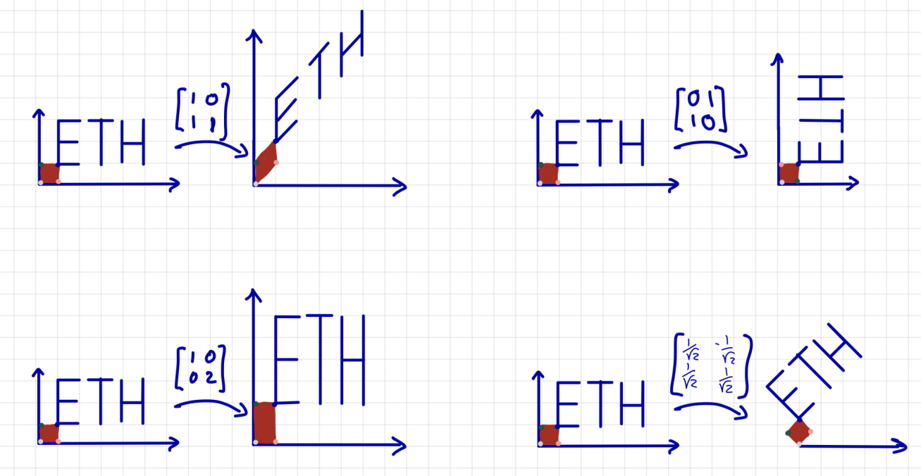
To understand in what ways a matrix transforms a vector we are specifically interested in the standard unit vectors $\textbf{e}_1, \textbf{e}_2, \dots, \textbf{e}_n$. To intuitively sum up why, it is because we can express everything in a space $\mathbb{R}^n$ using the set of standard unit vectors. If we know what $A$ does to this set of vectors, we can generalize the effect of $A$ to all vectors in $\mathbb{R}^n$.

This is demonstrated below. If you know what happens to the unit square (little red guy), then you can generalize that effect to any other shape or e.g. to any set of vectors.

Example from HS23

Certain operations have special names that intuitively describe the operation a matrix does. Some examples are scaling, shear, rotation and projection.

Hints

1. In-Class

2. Section 2.1.4 from the lecture notes is helpful.

3. a) You can try to visualize this on unit vectors in $\R^3$. You can also first consider the matrix

   $$\begin{bmatrix} \frac1{\sqrt2} & -\frac1{\sqrt2} \\ \frac1{\sqrt2} & \frac1{\sqrt2} \end{bmatrix}$$

4. No hints.

5. No hints.

6. d) Write the matrix $A \in \R^{3\times 3}$ in a generic way. Remember that if you can find one vector other than $\textbf{0}$ with $A\textbf{x} = \textbf{0}$, then you can prove $\textbf{rank}(A) \le 2$.

7. No hints.